Machine learning algorithms have revolutionized data analysis, enabling businesses and researchers to make highly accurate predictions based on vast datasets. Among these, the Random Forest algorithm stands out as one of the most versatile and powerful tools for classification and regression tasks.
This article will explore the key concepts behind the Random Forest algorithm, its working principles, advantages, limitations, and practical implementation using Python. Whether you’re a beginner or an experienced developer, this guide provides a comprehensive overview of Random Forest in action.
Key Takeaways
- The Random Forest algorithm combines multiple trees to create a robust and accurate prediction model.
- The Random Forest classifier combines multiple decision trees using ensemble learning principles, automatically determines feature importance, handles classification and regression tasks effectively, and seamlessly manages missing values and outliers.
- Feature importance rankings from Random Forest provide valuable insights into your data.
- Parallel processing capabilities make it efficient for large sets of training data.
- Random Forest reduces overfitting through ensemble learning and random feature selection.
What Is the Random Forest Algorithm?
The Random Forest algorithm is an ensemble learning method that constructs multiple decision trees and combines their outputs to make predictions. Each tree is trained independently on a random subset of the training data using bootstrap sampling (sampling with replacement).
Additionally, at each split in the tree, only a random subset of features is considered. This random feature selection introduces diversity among trees, reducing overfitting and improving prediction accuracy.
The concept mirrors the collective wisdom principle. Just as large groups often make better decisions than individuals, a forest of diverse decision trees typically outperforms individual decision trees.
For example, in a customer churn prediction model, one decision tree may prioritize payment history, while another focuses on customer service interactions. Together, these trees capture different aspects of customer behavior, producing a more balanced and accurate prediction.
Similarly, in a house price prediction task, each tree evaluates random subsets of the data and features. Some trees may emphasize location and size, while others focus on age and condition. This diversity ensures the final prediction reflects multiple perspectives, leading to robust and reliable results.
Mathematical Foundations of Decision Trees in Random Forest
To understand how Random Forest makes decisions, we need to explore the mathematical metrics that guide splits in individual decision trees:
1. Entropy (H)
Measures the uncertainty or impurity in a dataset.
- pi: Proportion of samples belonging to class
- c: Number of classes.
2. Information Gain (IG)
Measures the reduction in entropy achieved by splitting the dataset:

- S: Original dataset
- Sj: Subset after split
- H(S): Entropy before the split
3. Gini Impurity (Used in Classification Trees)
This ia an alternative to Entropy. Gini Impurity is computed as:

4. Mean Squared Error (MSE) for Regression
For Random Forest regression, splits minimize the mean squared error:

- yi: Actual values
- yˉ: Mean predicted value
Why Use Random Forest?
The Random forest ML classifier offers significant benefits, making it a robust machine learning algorithm among other supervised machine learning algorithms.
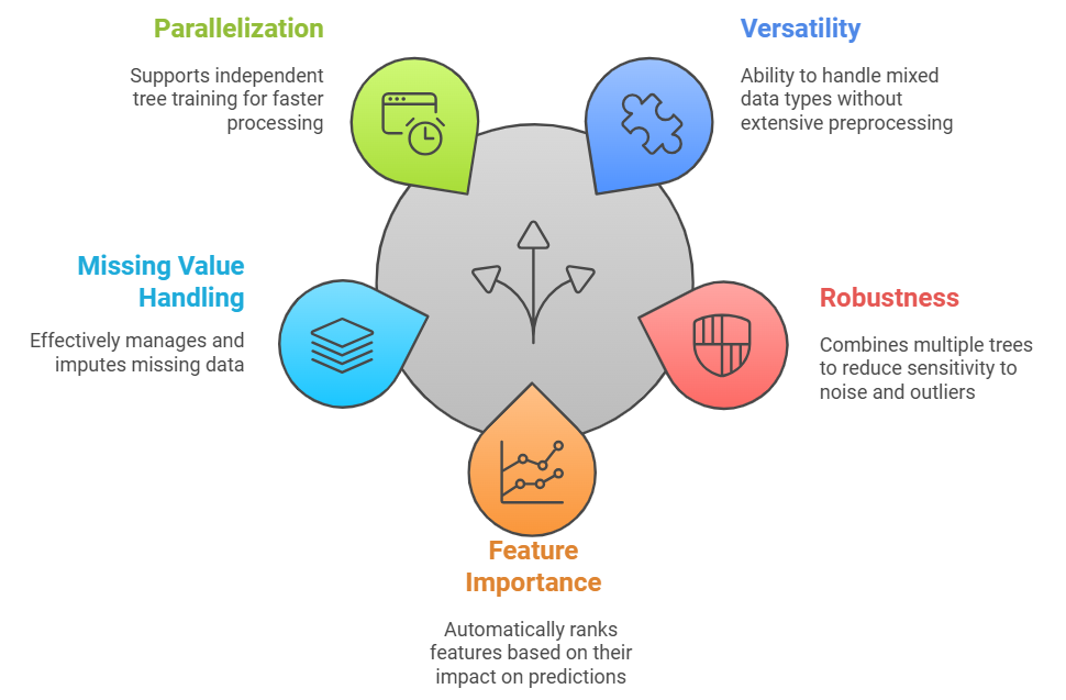
1. Versatility
- Random Forest model excels at simultaneously processing numerical and categorical training data without extensive preprocessing.
- The algorithm creates splits based on threshold values for numerical data, such as age, income, or temperature readings. When handling categorical data like color, gender, or product categories, binary splits are created for each category.
- This versatility becomes particularly valuable in real-world classification tasks where data sets often contain mixed data types.
- For example, in a customer churn prediction model, Random Forest can seamlessly process numerical features like account balance and service duration alongside categorical features like subscription type and customer location.
2. Robustness
- The ensemble nature of Random Forest provides exceptional robustness by combining multiple decision trees.
- Each decision tree learns from a different subset of the data, making the overall model less sensitive to noisy data and outliers.
- Consider a housing price prediction scenario and one decision tree might be influenced by a costly house in the dataset. However, because hundreds of other decision trees are trained on different data subsets, this outlier’s impact gets diluted in the final prediction.
- This collective decision-making process significantly reduces overfitting – a common problem where models learn noise in the training data rather than genuine patterns.
3. Feature Importance
- Random Forest automatically calculates and ranks the importance of each feature in the prediction process. This ranking helps data scientists understand which variables most strongly influence the outcome.
- The Random Forest model in machine learning measures importance by tracking how much prediction error increases when a feature is randomly shuffled.
- For instance, in a credit risk assessment model, the Random Forest model might reveal that payment history and debt-to-income ratio are the most crucial factors, while customer age has less impact. This insight proves invaluable for feature selection and model interpretation.
4. Missing Value Handling
- Random Forest effectively manages missing values, making it well-suited for real-world datasets with incomplete or imperfect data. It handles missing values through two primary mechanisms:
- Surrogate Splits (Replacement Splits): During tree construction, Random Forest identifies alternative decision paths (surrogate splits) based on correlated features. If a primary feature value is missing, the model uses a surrogate feature to make the split, ensuring predictions can still proceed.
- Proximity-Based Imputation: Random Forest leverages proximity measures between data points to estimate missing values. It calculates similarities between observations and imputes missing entries using values from the nearest neighbors, effectively preserving patterns in the data.
- Consider a scenario predicting whether someone will repay a loan. If salary information is missing, Random Forest analyzes related features, such as job history, past payments, and age, to make accurate predictions. By leveraging correlations among features, it compensates for gaps in data rather than discarding incomplete records.
5. Parallelization
- The Random Forest classifier architecture naturally supports parallel computation because each decision tree trains independently.
- This improves scalability and reduces training time significantly since tree construction can be distributed across multiple CPU cores or GPU clusters,
- Modern implementations, such as Scikit-Learn’s RandomForestClassifier, leverage multi-threading and distributed computing frameworks like Dask or Spark to process data in parallel.
- This parallelization becomes crucial when working with big data. For instance, when processing millions of customer transactions for fraud detection, parallel processing can reduce training time from hours to minutes.
Ensemble Learning Technique
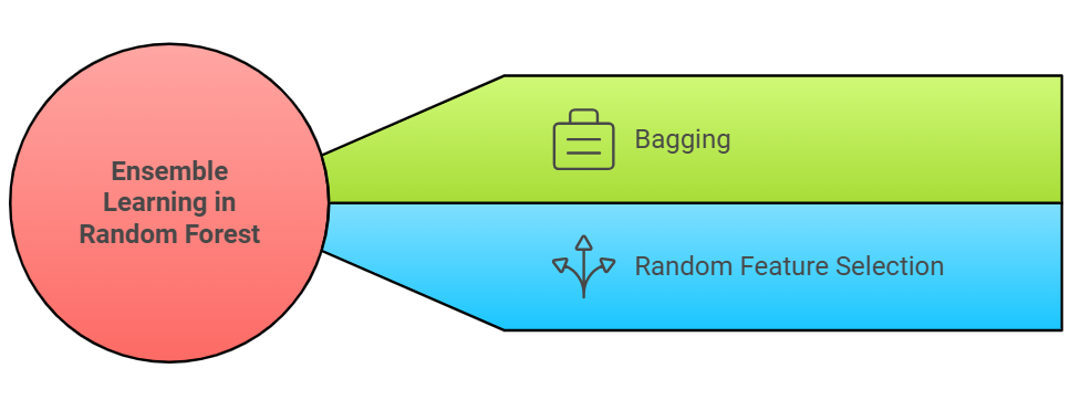
Ensemble learning in the Random Forest algorithm combines multiple decision trees to create more accurate predictions than a single tree could achieve alone. This approach works through two main techniques:
Bagging (Bootstrap Aggregating)
- Each decision tree is trained on a random sample of the data. It’s like asking different people for their opinions. Each group might notice different patterns, and combining their views often leads to better decisions.
- As a result, different trees learn slightly varied patterns, reducing variance and improving generalization.
Random Feature Selection
- At each split point in a decision tree, only a random subset of features is considered, rather than evaluating all features.
- This randomness ensures decorrelation between the trees, preventing them from becoming overly similar and reducing the risk of overfitting.
This ensemble approach makes machine learning Random Forest algorithm particularly effective for real-world classifications where data patterns are complex, and no single perspective can capture all-important relationships.
Variants of Random Forest Algorithm
Random Forest method has several variants and extensions designed to address specific challenges, such as imbalanced data, high-dimensional features, incremental learning, and anomaly detection. Below are the key variants and their applications:
1. Extremely Randomized Trees (Extra Trees)
- Uses random splits instead of finding the best split.
- Best for high-dimensional data that require faster training rather than 100% accuracy.
2. Rotation Forest
- Applies Principal Component Analysis (PCA) to transform features before training trees.
- Best for multivariate datasets with high correlations among features.
3. Weighted Random Forest (WRF)
- Assigns weights to samples, prioritizing hard-to-classify or minority class examples.
- Best for imbalanced datasets like fraud detection or medical diagnosis.
4. Oblique Random Forest (ORF)
- Uses linear combinations of features instead of single features for splits, enabling non-linear boundaries.
- Best for tasks with complex patterns such as image recognition.
5. Balanced Random Forest (BRF)
- Handles imbalanced datasets by over-sampling minority classes or under-sampling majority classes.
- Best for binary classification with skewed class distributions (e.g., fraud detection).
6. Totally Random Trees Embedding (TRTE)
- Projects data into a high-dimensional sparse binary space for feature extraction.
- Best for unsupervised learning and preprocessing for clustering algorithms.
7. Isolation Forest (Anomaly Detection)
- Focuses on isolating outliers by random feature selection and splits.
- Best for anomaly detection in fraud detection, network security, and intrusion detection systems.
8. Mondrian Forest (Incremental Learning)
- Supports incremental updates, allowing dynamic learning as new data becomes available.
- Best for streaming data and real-time predictions.
9. Random Survival Forest (RSF)
- Designed for survival analysis, predicting time-to-event outcomes with censored data.
- Best for medical research and patient survival predictions.
How Does Random Forest Algorithm Work?
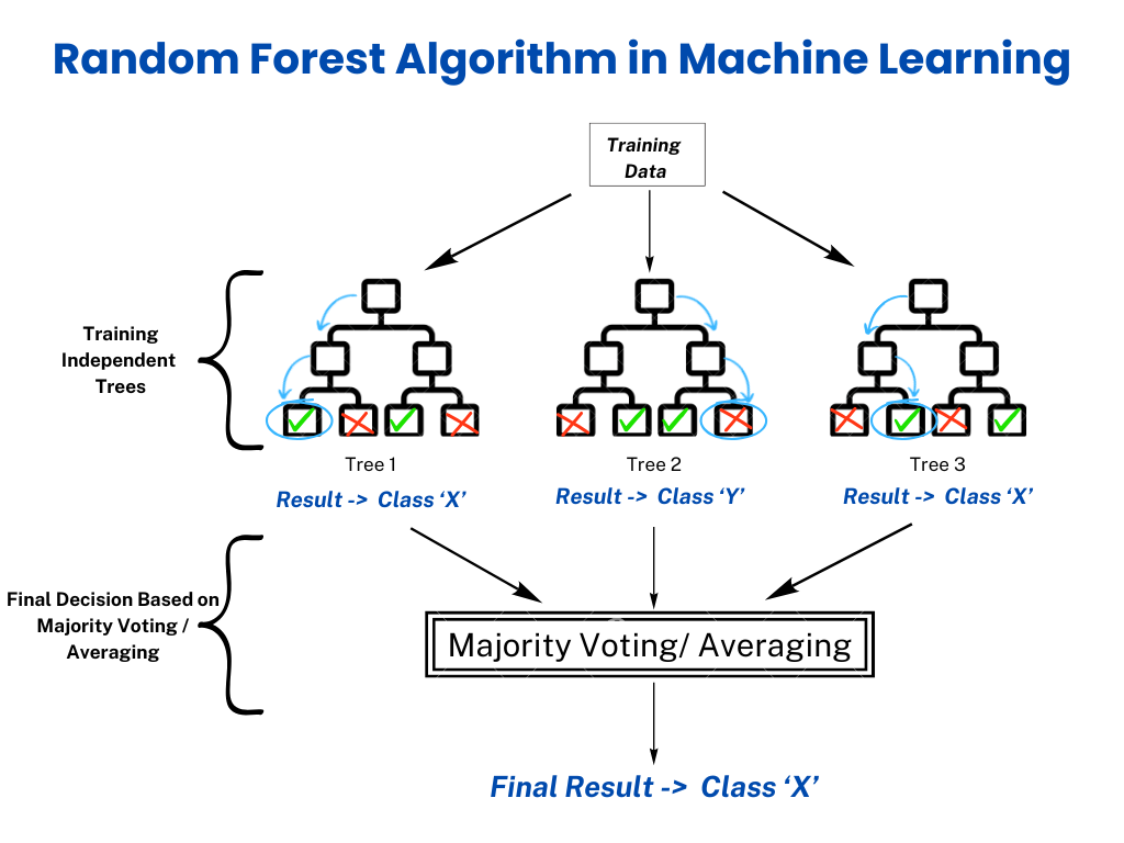
The Random Forest algorithm creates a collection of decision trees, each trained on a random subset of the data. Here’s a step-by-step breakdown:
Step 1: Bootstrap Sampling
- The Random Forest algorithm uses bootstrapping, a technique for generating multiple datasets by random sampling (with replacement) from the original training dataset. Each bootstrap sample is slightly different, ensuring that individual trees see diverse subsets of the data.
- Approximately 63.2% of the data is used in training each tree, while the remaining 36.8% is left out as out-of-bag samples (OOB samples), which are later used to estimate model accuracy.
Step 2: Feature Selection
- A decision tree randomly selects a subset of features rather than all features for each split, which helps reduce overfitting and ensures diversity among trees.
- For Classification: The number of features considered at each split is set to:
m = sqrt(p) - For Regression: The number of features considered at each split is:
m = p/3where:- p = total number of features in the dataset.
- m = number of features randomly selected for evaluation at each split.
Step 3: Tree Building
- Decision trees are constructed independently using the sampled data and the chosen features. Each tree grows until it reaches a stopping criterion, such as a maximum depth or a minimum number of samples per leaf.
- Unlike pruning methods in single decision trees, Random Forest trees are allowed to fully grow. It relys on ensemble averaging to control overfitting.
Step 4: Voting or Averaging
- For classification problems, each decision tree votes for a class, and the majority vote determines the final prediction.
- For regression problems, the predictions from all trees are averaged to produce the final output.
Step 5: Out-of-Bag (OOB) Error Estimation (Optional)
- The OOB samples, which were not used to train each tree, serve as a validation set.
- The algorithm computes OOB error to assess performance without requiring a separate validation dataset. It offers an unbiased accuracy estimate.
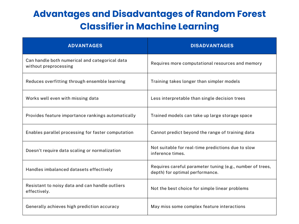
Advantages and Disadvantages of the Random Forest Classifier
The Random Forest machine learning classifier is regarded as one of the most powerful algorithms due to its ability to handle a variety of data types and tasks, including classification and regression. However, it also comes with some trade-offs that need to be considered when choosing the right algorithm for a given problem.
Advantages of Random Forest Classifier
- Random Forest can process both numerical and categorical data without requiring extensive preprocessing or transformations.
- Its ensemble learning technique reduces variance, making it less prone to overfitting than single decision trees.
- Random Forest can represent missing data or make predictions even when some feature values are unavailable.
- It provides a ranking of feature importance providing insights into which variables contribute most to predictions.
- The ability to process data in parallel makes it scalable and efficient for large datasets.
Disadvantages of Random Forest Classifier
- Training multiple trees requires more memory and processing power than simpler models like logistic regression.
- Unlike single decision trees, the ensemble structure makes it harder to interpret and visualize predictions.
- Models with many trees may occupy significant storage space, especially for big data applications.
- Random Forest may have slow inference times. This may limit its use in scenarios requiring instant predictions.
- Careful adjustment of hyperparameters (e.g., number of trees, maximum depth) is necessary to optimize performance and avoid excessive complexity.
The table below outlines the key strengths and limitations of the Random Forest algorithm.
Random Forest Classifier in Classification and Regression
The algorithm for Random Forest adapts effectively to classification and regression tasks by using slightly different approaches for each type of problem.
Classification
In classification, a Random Forest uses a voting system to predict categorical outcomes (such as yes/no decisions or multiple classes). Each decision tree in the forest makes its prediction, and a majority vote determines the final answer.
For example, if 60 trees predict “yes” and 40 predict “no,” the final prediction will be “yes.”
This approach works particularly well for problems with:
- Binary classification (e.g., spam vs. non-spam emails).
- Multi-class classification (e.g., identifying species of flowers based on petal dimensions).
- Imbalanced datasets, where class distribution is uneven due to its ensemble nature, reduce bias.
Regression
Random Forest employs different methods for regression tasks, where the goal is to predict continuous values (like house prices or temperature). Instead of voting, each decision tree predicts a specific numerical value. The final prediction is calculated by averaging all these individual predictions. This method effectively handles complex relationships in data, especially when the connections between variables aren’t straightforward.
This approach is ideal for:
- Forecasting tasks (e.g., weather predictions or stock prices).
- Non-linear relationships, where complex interactions exist between variables.
Random Forest vs. Other Machine Learning Algorithms
The table highlights the key differences between Random Forest and other machine learning algorithms, focusing on complexity, accuracy, interpretability, and scalability.
| Aspect | Random Forest | Decision Tree | SVM (Support Vector Machine) | KNN (K-Nearest Neighbors) | Logistic Regression |
| Model Type | Ensemble method (multiple decision trees combined) | Single decision tree | Non-probabilistic, margin-based classifier | Instance-based, non-parametric | A probabilistic, linear classifier |
| Complexity | Moderately high (due to the ensemble of trees) | Low | High, especially with non-linear kernels | Low | Low |
| Accuracy | High accuracy, especially for large datasets | Can overfit and have lower accuracy on complex datasets | High for well-separated data; less effective for noisy datasets | Dependent on the choice of random k and distance metric | Performs well for linear relationships |
| Handling Non-Linear Data | Excellent, captures complex patterns due to tree ensembles | Limited | Excellent with non-linear kernels | Moderate, depends on k and data distribution | Poor |
| Overfitting | Less prone to overfitting (due to averaging of trees) | Highly prone to overfitting | Susceptible to overfitting with non-linear kernels | Prone to overfitting with small k; underfitting with large k | Less prone to overfitting |
Key Steps of Data Preparation for Random Forest Modeling
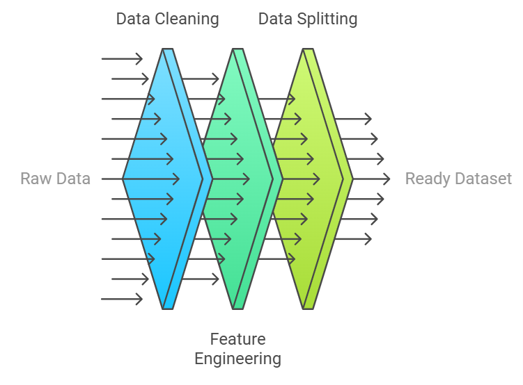
Adequate data preparation is crucial for building a robust Random Forest model. Here’s a comprehensive checklist to ensure optimal data readiness:
1. Data Cleaning
- Use imputation techniques like mean, median, or mode for missing values. Random Forest can also handle missing values natively through surrogate splits.
- Use boxplots or z-scores and decide whether to remove or transform outliers based on domain knowledge.
- Ensure categorical values are standardized (e.g., ‘Male’ vs. ‘M’) to avoid errors during encoding.
2. Feature Engineering
- Combine features or extract insights, such as age groups or time intervals from timestamps.
- Use label encoding for ordinal data and apply one-hot encoding for nominal categories.
3. Data Splitting
- Use an 80/20 or 70/30 split to balance the training and testing phases.
- In classification problems with imbalanced data, use stratified sampling to maintain class proportions in both training and testing sets.
How to Implement Random Forest Algorithm
Below is a simple Random Forest algorithm example using Scikit-Learn for classification. The dataset used is the built-in Iris dataset.
import numpy as np
import pandas as pd
from sklearn.datasets import load_iris
from sklearn.model_selection import train_test_split
from sklearn.ensemble import RandomForestClassifier
from sklearn.metrics import accuracy_score, classification_report, confusion_matrix
iris = load_iris()
X = iris.data
y = iris.target
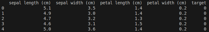
iris_df = pd.DataFrame(data=iris.data, columns=iris.feature_names)
iris_df['target'] = iris.target
print(iris_df.head())
X_train, X_test, y_train, y_test = train_test_split(X, y, test_size=0.3, random_state=42)
rf_classifier = RandomForestClassifier(n_estimators=100, random_state=42)
rf_classifier.fit(X_train, y_train)
y_pred = rf_classifier.predict(X_test)
accuracy = accuracy_score(y_test, y_pred)
print(f"Accuracy: {accuracy:.2f}")
print("\nClassification Report:")
print(classification_report(y_test, y_pred))
print("\nConfusion Matrix:")
print(confusion_matrix(y_test, y_pred))Explanation of the Code
Now, let’s break the above Random Forest algorithm in machine learning example into several parts to understand how the code works:
- Data Loading:
- The Iris dataset is a classic dataset in machine learning for classification tasks.
- X contains the features (sepal and petal measurements), and y contains the target class (species of iris). Here is the first five data rows in the Iris dataset.
- Data Splitting:
- The dataset is split into training and testing sets using train_test_split.
- Model Initialization:
- A Random Forest classifier is initialized with 100 trees (n_estimators=100) and a fixed random seed (random_state=42) for reproducibility.
- Model Training:
- The fit method trains the Random Forest on the training data.
- Prediction:
- The predict method generates predictions on the test set.
- Evaluation:
- The accuracy_score function computes the model’s accuracy.
- classification_report provides detailed precision, recall, F1-score, and support metrics for each class.
- confusion_matrix shows the classifier’s performance in terms of true positives, false positives, true negatives, and false negatives.
Output Example:
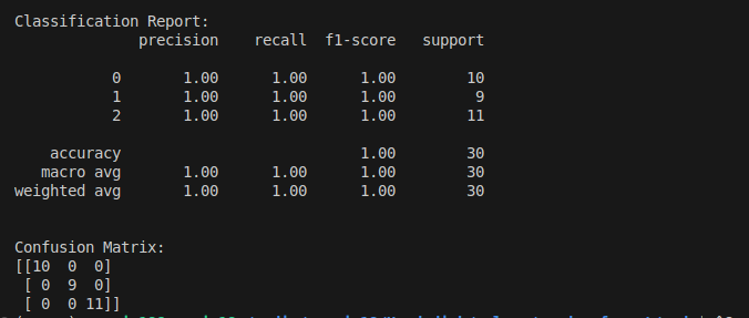
This example demonstrates how to effectively use the Random Forest classifier in Scikit-Learn for a classification problem. You can adjust parameters like n_estimators, max_depth, and max_features to fine-tune the model for specific datasets and applications.
Potential Challenges and Solutions When Using the Random Forest Algorithm
Several challenges may arise when using the Random Forest algorithm, such as high dimensionality, imbalanced data, and memory constraints. These issues can be mitigated by employing feature selection, class weighting, and tree depth control to improve model performance and efficiency.
1. High Dimensionality
Random Forest can struggle with datasets containing a large number of features, causing increased computation time and reduced interpretability.
Solutions:
Use feature importance scores to select the most relevant features.
importances = rf_classifier.feature_importances_Apply algorithms like Principal Component Analysis (PCA) or t-SNE to reduce feature dimensions.
from sklearn.decomposition import PCA
pca = PCA(n_components=10)
X_reduced = pca.fit_transform(X)
2. Imbalanced Data
Random Forest may produce biased predictions when the dataset has imbalanced classes.
Solutions:
Apply class weights. You can assign higher weights to minority classes using the class_weight=’balanced’ parameter in Scikit-Learn.
RandomForestClassifier(class_weight='balanced')Use algorithms like Balanced Random Forest to resample data before training.
from imblearn.ensemble import BalancedRandomForestClassifier
clf = BalancedRandomForestClassifier(n_estimators=100)
3. Memory Constraints
Training large forests with many decision trees can be memory-intensive, especially for big data applications.
Solutions:
- Reduce the number of decision trees.
- Set a maximum depth (max_depth) to avoid overly large trees and excessive memory usage.
- Use tools like Dask or H2O.ai to handle datasets too large to fit into memory.
A Real-Life Examples of Random Forest
Here are three practical applications of Random Forest showing how it solves real-world problems:
Retail Analytics
Random Forest helps predict customer purchasing behaviour by analyzing shopping history, browsing patterns, demographic data, and seasonal trends. Major retailers use these predictions to optimize inventory levels and create personalized marketing campaigns, achieving up to 20% improvement in sales forecasting accuracy.
Medical Diagnostics
Random Forest aids doctors in disease detection by processing patient data, including blood test results, vital signs, medical history, and genetic markers. A notable example is breast cancer detection, where Random Forest models analyze mammogram results alongside patient history to identify potential cases with over 95% accuracy.
Environmental Science
Random Forest predicts wildlife population changes by processing data about temperature patterns, rainfall, human activity, and historical species counts. Conservation teams use these predictions to identify endangered species and implement protective measures before population decline becomes critical.
Future Trends in Random Forest and Machine Learning
The evolution of Random Forest in machine learning continues to advance alongside broader developments in machine learning technology. Here’s an examination of the key trends shaping its future:
1. Integration with Deep Learning
- Hybrid models combining Random Forest with neural networks.
- Enhanced feature extraction capabilities.
2. Automated Optimization
- Advanced automated hyperparameter tuning
- Intelligent feature selection
3. Distributed Computing
- Improved parallel processing capabilities
- Better handling of big data
Conclusion
Random Forest is a robust model that combines multiple decision trees to make reliable predictions. Its key strengths include handling various data types, managing missing values, and identifying essential features automatically.
Through its ensemble approach, Random Forest delivers consistent accuracy across different applications while remaining straightforward to implement. As machine learning advances, Random Forest proves its value through its balance of sophisticated analysis and practical utility, making it a trusted choice for modern data science challenges.
FAQs on Random Forest Algorithm
1. What Is the Optimal Number of Trees for a Random Forest?
Good results typically result from starting with 100-500 decision trees. The number can be increased when more computational resources are available, and higher prediction stability is needed.
2. How Does Random Forest Handle Missing Values?
Random Forest effectively manages missing values through multiple techniques, including surrogate splits and imputation methods. The algorithm maintains accuracy even when data is incomplete.
3. What Techniques Prevent Overfitting in Random Forest?
Random Forest prevents overfitting through two main mechanisms: bootstrap sampling and random feature selection. These create diverse trees and reduce prediction variance, leading to better generalization.
4. What Distinguishes Random Forest from Gradient Boosting?
Both algorithms use ensemble methods, but their approaches differ significantly. Random Forest builds trees independently in parallel, while Gradient Boosting constructs trees sequentially. Each new tree focuses on correcting errors made by previous trees.
5. Does Random Forest Work Effectively with Small Datasets?
Random Forest performs well with small datasets. However, parameter adjustments—particularly the number of trees and maximum depth settings—are crucial to maintaining model performance and preventing overfitting.
6. What Types of Problems Can Random Forest Solve?
Random Forest is highly versatile and can handle:
- Classification: Spam detection, disease diagnosis, fraud detection.
- Regression: House price prediction, sales forecasting, temperature prediction.
7. Can Random Forest Be Used for Feature Selection?
Yes, Random Forest provides feature importance scores to rank variables based on their contribution to predictions. This is particularly useful for dimensionality reduction and identifying key predictors in large datasets.
8. What Are the Key Hyperparameters in Random Forest, and How Do I Tune Them?
Random Forest algorithms require careful tuning of several key parameters significantly influencing model performance. These hyperparameters control how the forest grows and makes decisions:
- n_estimators: Number of trees (default = 100).
- max_depth: Maximum depth of each tree (default = unlimited).
- min_samples_split: Minimum samples required to split a node.
- min_samples_leaf: Minimum samples required at a leaf node.
- max_features: Number of features considered for each split.
9. Can Random Forest Handle Imbalanced Datasets?
Yes, it can handle imbalance using:
- Class weights: Assign higher weights to minority classes.
- Balanced Random Forest variants: Use sampling techniques to equalize class representation.
- Oversampling and undersampling techniques: Methods like SMOTE and Tomek Links balance datasets before training.
10. Is Random Forest Suitable for Real-Time Predictions?
Random Forest is not ideal for real-time applications due to long inference times, especially with a large number of trees. For faster predictions, consider algorithms like Logistic Regression or Gradient Boosting with fewer trees.
[ad_2]
Source link